Search
Sidebar Menu
AMMA


Wise Words
"Cherish your visions and your dreams as they are the children of your soul; the blue prints of your ultimate achievements."
- Napoleon Hill
Climate / Health analysis
The climate explorer developed at KNMI is a powerfull tool to perform climate related studies and complex statistical analysis on the data. This tool only requests an internet connection and a browser. The Climate Explorer system has the following structure. First you select a time series of climate data, either station data (by name or location), some climate index (e.g. NAO, NINO3), a region from a gridded field, or your own series. This data is presented, and can then be correlated with another time series, or with a field of data (gridded observations or some fields of the NCEP/NCAR reanalysis).
The outcome of the comparison is
- a plot of correlations if a field was selected (significance, slope and
intercept are also available)
- a yearly cycle of the first data set and the correlation and significance if
one or two time series were selected,
- a scatter plot and tercile plot if only one month or average over months was selected with a fixed lag
- a lag-correlation plot if only one month or average over months was selected
with a varying lag.
- a table of correlations and significances otherwise.
In the following a short tutorial is provided to highlight the basics of climate explorer. This is done in order to carry out climate / health impacts analysis.
1) Launch the web site and register
You will need to register first if you want to take advantage of all the climate explorer functions. By default, you log in as an anonymous user.After performing the registration form, add the webpage to your bookmarks/favorites to avoid logging in.
After logging in, you will get a welcome message. The main page (left-centre) generally displays the plots ans analysis outputs. On the right side, different links are available. These links allow downloading climate/meteorological stations data and doing the analysis.
2) Dowload/plot data from the KNMI climate explorer. Three examples to start.
First, If you want download the data in order to do the analysis with your favorite software. Let's describe few examples as a starting point. Note that examples are also provided on climate explorer.2.1 Download and plot rainfall daily station data
In "select a time serie" click on "daily station data".
Then different datas are available (GHCN, ECA...). An hyperlink is generally given for each dataset if you want to know more details about it.
Fill the box precipitation below GHCN.
The select tab allows different way of getting the station you're interested in. You can browse for the station name, you can retrieve N stations (10 by default) within a rectangular box, displays all the station in a lat-lon rectangular box, or browse by station number.
Let's display all the station between 10N and 15N and 16W and 16E.
Type all station in the region: 10N 15N -16E 16E.
Then a list of station appears. Select for example KITA (mali) by clicking on the related link "get data".
Climate explorer will plot the rainfall time serie, two annual cycles and anomalies with respect to the annual cycle. At this point you can get the plots in postscripts format, or gif if you "save the image as" in the browser. Then you can download the data as well, by clicking on "raw data" (ASCII outputs, easy to copy and paste in excel for example) or in netcdf format.
If you click on "raw data" at this point you will see the data sorted in four columns: YEAR MONTH DAY RAINFALL_VALUE. Then, you can copy and paste the values to a text file.
You can reduce the time period if you want by selecting years 1980 1999, then press select for example.
2.2 Extract, dowload and plot daily rainfall from a gridded dataset (ERA40 reanalysis for example)
In "Select a field" select "Daily fields". Then you will see a list of observation, reanalysis and different climate models used for the IPCC AR4 report.
Click the box "prcp" in ERA40 then press enter. Different options are now available. You can extract a time serie by averaging the grid points within a rectangular box or a set of grid points. You can also compute a new field (computing monthly seasonal means etc etc) and you can apply a time filter.
In extract time series select the latitude range 10N-20N and -16E and 16E. Then click on make time series. The time serie appears (average of daily rainfall for ERA40 between 10N-20N, 16W-16E) and you can retrieve the data and the plots as previously mentioned.
2.3 Upload, plot and analyzing your own data time serie
Let's now upload your own data. As an example, we will upload the number of yearly reported cases of yellow fever over Ghana (from WHO dataset).
The yearly data sorted in two columns (year / number of reported cases) can be accessed here. Blank values must be replaced by -999 (missing data).
In climate explorer select "upload your own time serie" . Details about the data formatting are displayed in the text box (generally multicolumn data with YEAR MONTH DAY VALUE standard).
Now copy and paste the yellow fever data in this box. Fill the name value in the upper box (yellow_fever_ghana for example), and select type: something different. When it is done click upload.
Then you will see the yellow fever plot:
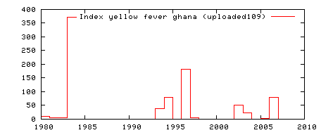
Your time serie has been successfully uploaded on climate explorer and can be accessed again under "user defined time serie". The field name is yellow_fever_ghana. This field will be stored for three days and then will be erased form the KNMI server.
Now we will try to correlate the yellow fever cases over Ghana with global sea surface temperature. First we must build yearly SST values using monthly means (the time scale must be consistent between both yellow fever and SST data). In "select a field" click "Monthly observations". Fill the SST box associated with the 1870-now: HadISST1 1° reconstruction, then press enter. In "Create a field with derived data" create the SST yearly means by pressing the tab Make new field (new time scale = annual, new variable = mean, threshold = no cut).
Wait the time to process the new field values. When it's over click again on "user defined time serie" and select again yellow_fever_ghana. In "Investigate this time serie" select Correlate with a field (correlation, regression composite). Fill the box "annual mean of monthly SST HadISST1" (the data you processed just before). Then click the Correlate tab or press enter. You will get the correlation map between global yearly SST and the reported cases of yellow fever over Ghana for the period 1980-2007 (you can save the image using "save image as" with a right click on the image.)
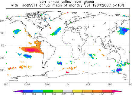
Strong positive correlations are shown in the tropical Pacific ocean (a pattern closed to the ENSO, but restricted to the eastern part of the basin).
3) The introduction section:
The introduction section provides News, examples, publication that use climate explorer to perform the analysis.4) The "select a time series" section
Here you can plot, download daily/monthly time series for both stations, predefined indices, or upload your own time serie. Note that the uploaded files will be available for three days on your account under user defined time serie. When you select a time serie (when the plots are displayed), you can:- in "Manipulate this time serie": you can generally change the time window, apply a high or a low pass filter , compute the time derivative.
- in "Create a lower resolution time serie" you can change the time resolution (daily to monthly, yearly etc etc...)
- correlate it with another time serie
- correlate it with a field (Rainfall, SST etc etc for various climate data)
- verify it with respect to another time serie
- Compute a spectrum
- Compute a Wavelet analysis
- Running mean/s.d./skew/curtosis
- Plot the linear fit and the probability density function
5) The "select a field" section
Here you can also plot, download daily/monthly time series for both stations, predefined indices, gridded data or upload your own field. Note that the uploaded files and processed fields (if you change the time scale from monthly to yearly for example) will be available for three days on your account under user defined time field.Here you always can:
- Extract a time serie from the gridded data, by averaging the values in a rectangular box, or you can retrieve alll the grid points inside a box.
- Create a new field with derived data . You can change the time resolution (monthly to yearly etc). This step must be done for example if you want to correlate a montly field with a yearly time serie for example see 2.3.
- You can plot the map (mean, variance, for a given year...)
- You can plot the difference with another field
- Compute the mean / extremes
- Correlate the field with a time serie
- Pointwise / spatial correlation with another 2D field
- Verify against observed data
- Makes EOFs
6) The "user-defined" subsection
For both time series and fields, your data will be stored in the user defined section. Give a name to your data to be sure to find what you've already done. The data are stored for 3 days. All the time processed files are stored there as well (for example if you build a monthly mean from daily values, the monthly data will be stored there).7) To avoid the bugs:
BE CAREFULL: EVERY TIME YOU MANIPULATE A FIELD/TIME SERIE AND COMPAIR/CORRELATE IT WITH ANOTHER ONE BE SURE THAT BOTH FIELDS HAVE THE SAME TIME SCALE (DAILY VS DAILY, YEARLY VS YEARLY...). OTHERWISE IT WON'T WORK!!!!!
Now play with climate explorer, it is really intuitive and easy to learn!!!
If you have any questions and/or feedbacks:
See the homepage of dr. Geert Jan van Oldenborgh
Or Email me